Lecture 20: Similar Matrices

20.1 Matrix Similarity

20.1.1 Definition of Similarity Matrices

#####Definition: Thematrixissimilar

description: let A and B be two n-order square matrices. If there exists a n-order invertible matrix P such that $P^{-1}AP=B$, then A is similar to B and denoted as A~B

Explanation

• Concept:
• If all are assumed to be matrix;
• Equivalence matrix: PAQ=B `<-` Isomorphic matrices: P and Q are unrelated;
• Similarity matrix: $P^{-1}AP=B$ <- Equivalence matrix: P and P inverse, the effect produced by their pincer interaction yields B;
• -> Therefore, similar matrices must also be equivalent
• Formula:
• A~A: Reflexivity
• If A~A, then B~A: symmetry
• If A~B,B~C, then A~C: transitivity -> proves A~C. You can first find A to B, then B to C, thus obtaining A to C;
• Supplement:
• Every matrix has an ideal matrix and its similarity <-> transitivity;

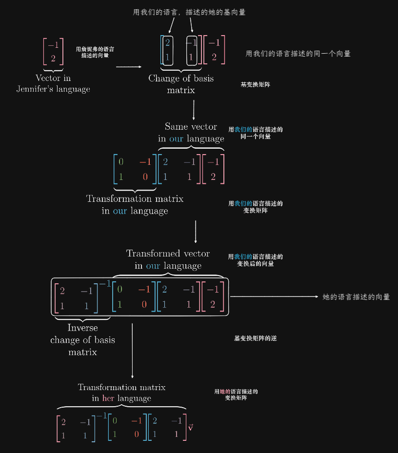
Supplement: Similarity matrices and $A^{-1}MA$

• Meaning:
• $A^{-1}MA$ Expressions imply mathematical transfer effects;
• The middle matrix represents a transformation you have seen, while the two outer matrices represent the transformation, i.e., the transformation on the viewpoint;
• The matrix product still representsthe same transformation, but from the perspective of others -> matrices A and B are similar, but the basis vectors differ;
• Illustration:
• 

20.1.2 Properties of Similar Matrices

Concept: The six main properties of the similarity matrix

• Note:
• The above six conditions are necessary for matrix similarity; if either is not met, the two matrices are not similar;
• However, even if 1~6 holds, it cannot be said that A is similar to B;
• Supplement:
• Concept:
• Under similarity transformations, the sum of the principal minors of each order is invariant.
• Example:
• For $A=\begin{bmatrix}1&1&0\\0&1&1\\1&0&1\end{bmatrix}$, the sum of the second-order principal minors is $1+1+1=3$.
• For $B=\begin{bmatrix}1&1&-1\\0&1&0\\1&0&1\end{bmatrix}$, the sum of the second-order principal minors is $1+2+1=4$.
• Therefore, A and B are not similar;

20.1.3 Important Conclusions of the Similarity Matrices

Concept: Conclusion One

• $$\text{ If }A\sim B,\text{ then }A^{k}\sim B^{k},f\left(A\right)\sim f\left(B\right)\left(\text{ where }f\left(x\right)\text{ is a polynomial }\right)$$

Concept: Conclusion two

• $$\text{If }A\sim B\text{ and }A\text{ is invertible, then }A^{-1}\sim B^{-1}\text{ and }f\left(A^{-1}\right)\sim f\left(B^{-1}\right),\text{ where }f\text{ is a polynomial}.$$

Concept: Conclusion three

• $$\text{If }A\sim B,\text{ then }A^\sim B^.$$

Concept: Conclusion Four

• $$\text{If }A\sim B,\text{ then }A^T\sim B^T.$$

Concept: Conclusion Five

• $$\text{ If }A\sim C,B\sim D,\text{ then }\begin{bmatrix}A&O\\O&B\end{bmatrix}\sim\begin{bmatrix}C&O\\O&D\end{bmatrix}$$

Analysis: Conclusion 1~3

• Because the means from A -> B are consistent in 1~3, their combinations are: $aA^{*}+bA^{-1}+cf\left(A\right)$ plus $P^{-1}$ and $P$:
• $$P^{-1}(aA^{}+bA^{-1}+cf\left(A\right))P=aB^{}+bB^{-1}+cf\left(B\right)$$

Analysis: Conclusion 4

• $A\sim B, $ then there is an invertible matrix $P, $ such that $P^{-1}AP=B, $ takes the transpose on both sides $, $ has $P^TA^T(P^{-1})^T=B^T$
• $P^{T}A^{T}\left(P^{T}\right)^{-1}=B^{T}$, so $A^{T}\sim B^{T}$. The similarity transformation used here differs from those in conclusions (1)–(3).

20.1.4 Identification and Proof of Similarity Between Two Matrices

Method: Definition method

• If there is an invertible matrix $P, $ such that $P^{-1}AP=B, $ then $A\sim B.$

Method: Utilize transitivity

• If A~V and V~B, then A~B

Method: Nature of use

• The nature of use can only deny the similarity between A and B, but cannot prove their similarity;
• Supplement:
• Under conditions A~B, properties can be used to find parameters in reverse, but as mentioned earlier, all properties are only necessary conditions for A~B

20.2 Similar Diagonalization of Matrices

20.2.1 Basic Concepts

#####Definition: Similardiagonalizationofmatrices

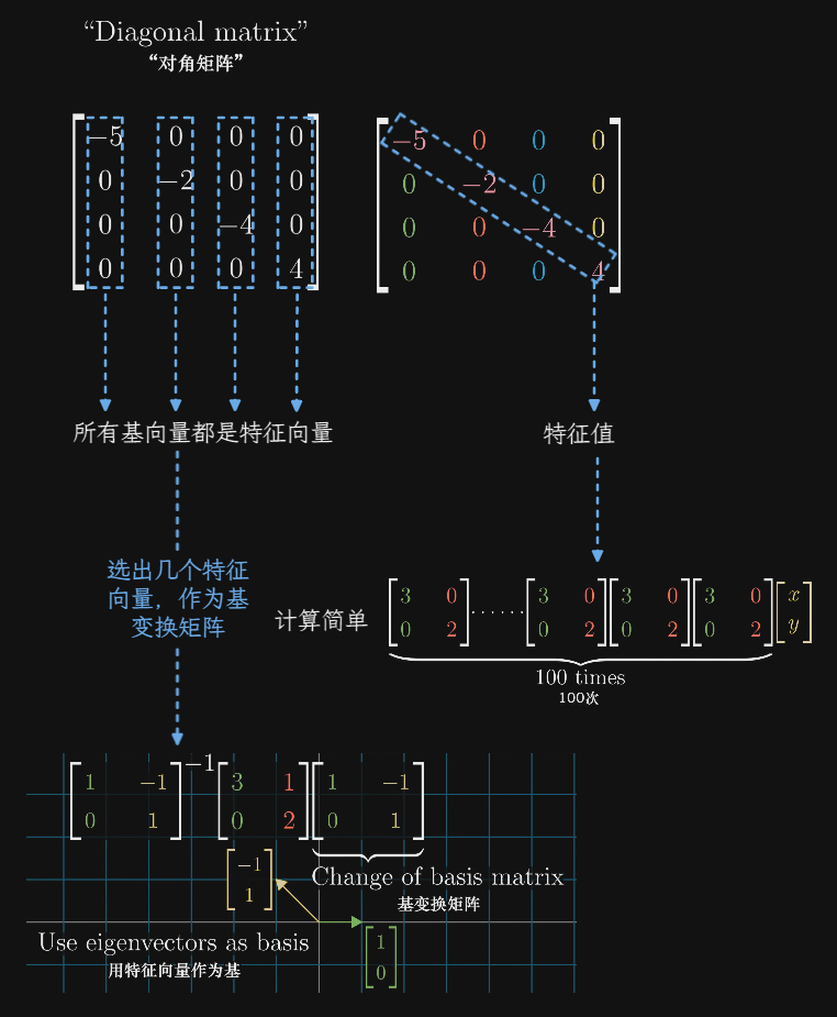
Description: Let A n order matrix. If there exists a P of n invertible matrix such that $P^{-1}AP=\Lambda$, then $\Lambda$ is a diagonal matrix, and A is called similarly diagonalizable as $A\sim\Lambda$, and $\Lambda$ is called the A similarity canonical form;

A The most essential definition is: A There are n linearly independent eigenvectors;

Concept: Graphic explanation

Concept: Conditions for Similar Diagonalization - Conclusion One

• -> Suppose: A can be similarly diagonalized
• -> There exists an invertible matrix P such that $P^{-1}AP=\Lambda$
• -> There exists an invertible matrix $P=(\xi_1,\xi_2)$ such that $AP=P\Lambda$
• -> There exists an invertible matrix $P=(\xi_1,\xi_2)$ such that $A(\xi_1,\xi_2)=(\xi_1,\xi_2)\Lambda$
• -> There exists an invertible matrix $P=(\xi_1,\xi_2)$ such that $(A\xi_1,A\xi_2)=(\lambda\xi_1,\lambda\xi_2)$
• -> There exists an invertible matrix $P=(\xi_1,\xi_2)$ such that $A\xi_i=\lambda\xi_i$
• -> So we get eigenvalues and eigenvectors: $A\xi_i=\lambda\xi_i$
• -> The column vectors that make up P are eigenvectors
• -> Conclusion:
• 1. A There are n linearly independent eigenvectors;
• 2. $P=[\xi_1, \xi_2, \cdots, \xi_n]$
• 3. $\Lambda=\begin{bmatrix}\lambda_1&&&&\\&\lambda_2&&&\\&&\ddots&&\\&&&\lambda_n\end{bmatrix}$
• 4. $$P^{-1}AP=\Lambda \quad\quad\rightarrow\quad\quad [\xi_1, \xi_2, \cdots, \xi_n]^{-1}A[\xi_1, \xi_2, \cdots, \xi_n]=\begin{bmatrix}\lambda_1&&&&\\&\lambda_2&&&\\&&\ddots&&\\&&&\lambda_n\end{bmatrix}$$
• This is a necessary condition;

Concept: Conditions for Similar Diagonalization - Conclusion Two

• Conclusion: If the n-order matrix A can be similarly diagonalized $\rightarrow$ $A$ corresponds to each $k_i$ eigenvalues with $k_i$ linearly independent eigenvectors;
• This is a necessary condition;

Concept: Conditions for similar diagonalization - Conclusion Three

• Conclusion: If the n-order matrix A has n different eigenvalues, $\rightarrow$ A can be similarly diagonalized;
• -> All are single roots with inherent linear independence, so similar diagonalization is possible;
• This is a sufficient condition

Concept: Conditions for similar diagonalization - Conclusion Four

• Conclusion: If the n-order matrix A is a real symmetric matrix $\rightarrow$ A can be similarly diagonalized;
• This is a sufficient condition

Concept: Other similar important conclusions

• Conclusion - If $A\sim\Lambda$, then every column in $P$ is an eigenvector of the A matrix, and these eigenvectors must be linearly independent;
• Conclusion - If $A\xi_i=\lambda_i\xi_i$, $\xi_i(i=1,2,3)$ constitutes $\Lambda$, then $A\sim\Lambda$
• Conclusion: Self-produced and self-sold
• Given a matrix A satisfying $\lambda$ and $\xi$, and n linearly independent eigenvectors, then $P^{-1}AP=\Lambda$ and $P=(\xi_1,\xi_2...\xi_n)$

20.2.2 Solving Similar Diagonalization

Method: Based on $P^{-1}AP=\Lambda$, find P steps

• Steps:
• 1. Because $|\lambda E-A|=0$, write the determinant $|\lambda E-A|$ and find the $\lambda_1,\lambda_2,\lambda_3,...\lambda_i$ of $A$
• 2. Find the stepped matrix of A for the corresponding $\lambda_1,\lambda_2,\lambda_3,...\lambda_i$, and from this find the eigenvector $\xi_1,\xi_2...\xi_i$ of A
• 3. Based on the properties of eigenvectors and eigenvalues, determine whether the current eigenvector is n linearly independent vectors. If so, combine the solved $\xi_i$ to get $P$:
• $P^{-1}AP=\Lambda=\begin{bmatrix}\lambda_1&&&&\\&\lambda_2&&&\\&&\ddots&&\\&&&\lambda_n\end{bmatrix}$
• Note:
• The eigenvector $\boldsymbol{\xi}_i$ in the $i$th column of $P$ must correspond to the eigenvalue $\lambda_i$ in $\Lambda$. The matrix $P$ is not unique.

Method: Derive $A$ from eigenvalues and eigenvectors

• Method:
• If an invertible matrix $P$ satisfies $P^{-1}AP=\Lambda$, then $A=P\Lambda P^{-1}$. This is the basic reconstruction formula.
• Example:
• -> $(\xi_{1},\xi_{2})^{-1}A(\xi_{1},\xi_{2})=(\begin{matrix}\lambda_{1}&0\\0&\lambda_{2}\end{matrix})$
• -> $A=(\xi_{1},\xi_{2})(\begin{matrix}\lambda_{1}&0\\0&\lambda_{2}\end{matrix})(\xi_{1},\xi_{2})^{-1}$

Method: Find $A^k$ and $f(A)$

• $$P^{-1}A^kP=\Lambda^k,\qquad A^k=P\Lambda^kP^{-1}=P\begin{bmatrix}\lambda_1^k&&&\\&\lambda_2^k&&\\&&\ddots&\\&&&\lambda_n^k\end{bmatrix}P^{-1}$$
• $$P^{-1}f(A)P=f(\Lambda),\qquad f(A)=Pf(\Lambda)P^{-1}=P\begin{bmatrix}f(\lambda_1)&&&\\&f(\lambda_2)&&\\&&\ddots&\\&&&f(\lambda_n)\end{bmatrix}P^{-1}.$$

Supplement: Properties that remain valid for singular matrices

• If $|A|=0$, then $0$ is an eigenvalue of $A$, so $A$ is singular.
• For every $n\times n$ matrix, $|A^*|=|A|^{n-1}$.
• Others:
• $|A^{*}|=|A|^{n-1}$ holds for every $n\times n$ matrix.
• $\left(AB\right)^{}=B^{}A^{*}$ holds for square matrices $A$ and $B$ of the same order.
• When $A$ is singular:
• Suppose A has triple roots, and a eigenvalue 1;
• If you now add E:+E+A before A;
• So: $|(tE+A)^{*}|=|tE+A|^{n-1}.$
• When $t\rightarrow 0^+$, the original eigenvalues of t are not 0; they are all continuous functions -> $|A^{*}|=|A|^{n-1}$ t with respect to t;
• That is: $|A^{*}|=|A|^{n-1}$ holds for both inversibility and irreversibility;

20.2.3 Example

Example Question: Which of the following options cannot resemble a diagonal matrix:

• Title:
• $$\begin{aligned}\left(A\right)A=&\begin{bmatrix}0&0&1\\0&1&0\\1&0&0\end{bmatrix}&(\mathbf{B}) \boldsymbol{B}=&\begin{bmatrix}1&1&1\\0&2&2\\0&0&3\end{bmatrix}\\(\mathbf{C})\boldsymbol{C}=&\begin{bmatrix}1&-2&1\\2&-4&2\\1&-2&1\end{bmatrix}&(\mathbf{D})\boldsymbol{D}=&\begin{bmatrix}2&-1&2\\5&-3&3\\-1&0&-2\end{bmatrix}\end{aligned}$$
• Analysis
• A is clearly symmetric, so A is similar to a diagonal matrix;
• B has a clear step and exactly three distinct eigenvalues, so if the three single roots correspond to eigenvalues, they must be similarly diagonalized;
• C is a rank-one matrix, so for a double heel and a single root, you need to determine the number of eigenvectors corresponding to them separately. The number of repetitions in option C equals the number of linearly independent eigenvectors, so C is similar to a diagonal matrix;
• Analysis

20.3 Similar Diagonalization of Real Symmetric Matrices

20.3.1 Real Symmetric Matrices

#####Definition: Realsymmetricmatrix

Description: if $A^T=A$, then A is a symmetric matrix. If all elements in A are real numbers, then A is a real symmetric matrix;

(1) A is a real symmetric matrix, then the eigenvalues of A are real numbers, and the eigenvectors are real vectors (no proof needed);

(2) Eigenvectors of a real symmetric matrix that correspond to distinct eigenvalues are orthogonal: $\lambda_1\neq\lambda_2\Rightarrow\xi_1\perp\xi_2$. For a repeated eigenvalue, an orthonormal basis can be chosen within its eigenspace.

(3) For any n-th order real symmetric matrix A, there exists an n-th order orthogonal matrix Q such that $Q^{\mathrm{T}}AQ=Q^{-1}AQ=\begin{bmatrix}\lambda_1&&&\\&\lambda_2&&\\&&\ddots&\\&&&\lambda_n\end{bmatrix}$, where $\lambda_i$ are all eigenvalues of A;

Explanation

• Explanation (2):
• Every real symmetric matrix has an orthonormal basis of eigenvectors and is therefore orthogonally diagonalizable.
• Explanation (3):
• Review: A has n linearly independent -> A~$\Lambda$ -> $[\xi_1, \xi_2, \cdots, \xi_n]^{-1}A[\xi_1, \xi_2, \cdots, \xi_n]=\begin{bmatrix}\lambda_1&&&&\\&\lambda_2&&&\\&&\ddots&&\\&&&\lambda_n\end{bmatrix}$
• Since a symmetric matrix can unconditionally yield $A\sim\Lambda$, it can always form a $[\xi_1, \xi_2, \cdots, \xi_n]^{-1}A[\xi_1, \xi_2, \cdots, \xi_n]=\begin{bmatrix}\lambda_1&&&&\\&\lambda_2&&&\\&&\ddots&&\\&&&\lambda_n\end{bmatrix}$ situation;
• And the symmetric matrix can also yield a $[\xi_1, \xi_2, \cdots, \xi_n]^{T}A[\xi_1, \xi_2, \cdots, \xi_n]=\begin{bmatrix}\lambda_1&&&&\\&\lambda_2&&&\\&&\ddots&&\\&&&\lambda_n\end{bmatrix}$ situation;
• Supplement: orthogonal matrix
• $Q^T=Q^{-1}$
• $Q^TQ=E$
• Q is formed from an orthonormal basis; obtain it by orthogonalizing and normalizing the eigenvectors when necessary;
• For every real symmetric matrix $A$, there exists an orthogonal matrix $Q$ such that $Q^TAQ=\Lambda$;

20.3.2 Orthogonal Diagonalization of a Real Symmetric Matrix

Method: If $A$ is an $n\times n$ real symmetric matrix:

• 1. Find the eigenvalues $\lambda_1,\lambda_2,\cdots,\lambda_n$ of $A$;
• 2. Find corresponding eigenvectors $\xi_1,\xi_2,\cdots,\xi_n$;
• 3. Within each repeated-eigenvalue eigenspace, orthogonalize if necessary and normalize the eigenvectors to obtain $\eta_1,\eta_2,\cdots,\eta_n$;
• 4. Set $Q=[\eta_1,\eta_2,\cdots,\eta_n]$. Then $Q$ is orthogonal and
• $$Q^{-1}AQ=Q^{\mathrm{T}}AQ=\Lambda.$$