Lecture 21: Definition and Matrix Representation of Quadratic Forms

21.1 Definition and Matrix Representation of a Quadratic Form

Definition: quadratic-form

A homogeneous polynomial of degree two in $n$ variables is called a quadratic form. It is usually written as

\begin{aligned} f(x_1,x_2,\ldots,x_n) &=\sum_{i=1}^{n}\sum_{j=1}^{n}a_{ij}x_ix_j \\ &=x^{\mathrm T}Ax, \end{aligned}

where

A= \begin{bmatrix} a_{11}&a_{12}&\cdots&a_{1n}\\ a_{21}&a_{22}&\cdots&a_{2n}\\ \vdots&\vdots&\ddots&\vdots\\ a_{n1}&a_{n2}&\cdots&a_{nn} \end{bmatrix}, \qquad x= \begin{bmatrix} x_1\\x_2\\\vdots\\x_n \end{bmatrix}.

Explanation

The same quadratic form can be represented by different nonsymmetric matrices. To make the matrix representation unique, $A$ is conventionally taken to be real and symmetric.
When $A$ is symmetric, the coefficient of the cross term $x_ix_j\ (i\ne j)$ is $2a_{ij}$.
The rank of the quadratic form is the rank of its unique symmetric matrix: $\operatorname{rank}(f)=\operatorname{rank}(A)$.
Example of a nonsymmetric representation:
$f(x_1,x_2,x_3)=x_1^2+x_2^2+x_3^2+4x_1x_2$;
$f(x)=\begin{bmatrix}x_1&x_2&x_3\end{bmatrix}\begin{bmatrix}1&4&0\\0&1&0\\0&0&1\end{bmatrix}\begin{bmatrix}x_1\\x_2\\x_3\end{bmatrix}$.
Example of a symmetric representation:
$f(x_1,x_2,x_3)=2x_1^2+2x_2^2+2x_3^2-2x_1x_2-2x_2x_3+2x_1x_3$;
$f(x)=\begin{bmatrix}x_1&x_2&x_3\end{bmatrix}\begin{bmatrix}2&-1&1\\-1&2&-1\\1&-1&2\end{bmatrix}\begin{bmatrix}x_1\\x_2\\x_3\end{bmatrix}$.

21.2 Congruence Transformations

21.2.1 Invertible Linear Transformations

Definition: linear-transformation

For an $n$-variable quadratic form $f(x)=x^{\mathrm T}Ax$, make the linear change of variables $x=Cy$:

\begin{bmatrix} x_1\\x_2\\\vdots\\x_n \end{bmatrix} = \begin{bmatrix} c_{11}&c_{12}&\cdots&c_{1n}\\ c_{21}&c_{22}&\cdots&c_{2n}\\ \vdots&\vdots&\ddots&\vdots\\ c_{n1}&c_{n2}&\cdots&c_{nn} \end{bmatrix} \begin{bmatrix} y_1\\y_2\\\vdots\\y_n \end{bmatrix}.

If $C$ is invertible, equivalently $\det C\ne0$, then $x=Cy$ is called an invertible linear transformation. Substitution gives

f(Cy)=(Cy)^{\mathrm T}A(Cy) =y^{\mathrm T}(C^{\mathrm T}AC)y =y^{\mathrm T}By =g(y),

where $B=C^{\mathrm T}AC$.

21.2.2 Definition and Properties of Matrix Congruence

Definition: congruent-quadratic-forms

Let $A$ and $B$ be $n\times n$ matrices. If an invertible matrix $C$ exists such that

C^{\mathrm T}AC=B,

then $A$ and $B$ are congruent, written $A\cong B$. Their corresponding quadratic forms $f(x)$ and $g(y)$ are also called congruent.

Explanation

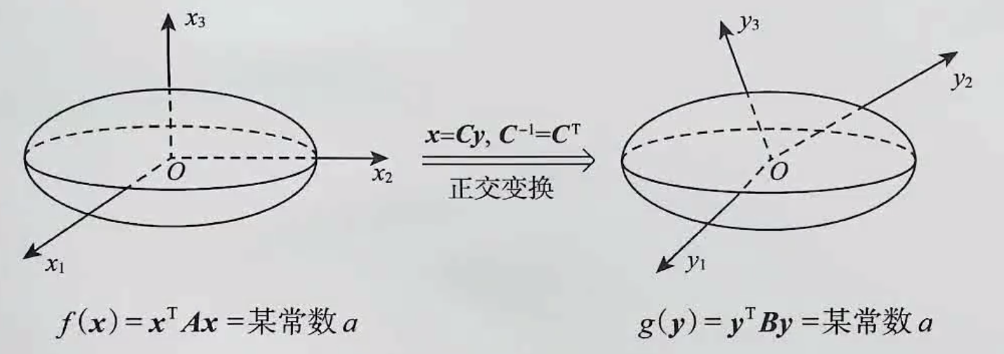
A congruence transformation is an invertible linear change of variables in a quadratic form.
For real symmetric matrices, congruence preserves symmetry, rank, and the positive and negative indices of inertia.
Left or right multiplication by an invertible matrix does not change rank, so $\operatorname{rank}(A)=\operatorname{rank}(B)$.
If $A=A^{\mathrm T}$, then

B^{\mathrm T} =(C^{\mathrm T}AC)^{\mathrm T} =C^{\mathrm T}A^{\mathrm T}C =C^{\mathrm T}AC =B.

Original example:

21.3 Standard and Canonical Forms

21.3.1 Definitions

Definition: standard-form

A quadratic form containing only squared terms and no cross terms is in standard form:

d_1y_1^2+d_2y_2^2+\cdots+d_ny_n^2.

Over the real numbers, further rescaling of variables changes every nonzero coefficient to $1$ or $-1$, producing the canonical form

y_1^2+\cdots+y_p^2-y_{p+1}^2-\cdots-y_{p+q}^2.

All remaining coefficients are zero. By Sylvester's law of inertia, the numbers $p$ and $q$ of positive and negative squared terms are invariant under congruence. The canonical form is therefore unique up to a permutation of variables.

21.3.2 Completing the Square and Orthogonal Transformations

Theorem: completing-the-square

Every real quadratic form $f(x)=x^{\mathrm T}Ax$ can be reduced to standard form by an invertible linear transformation $x=Cy$; rescaling the variables then gives the canonical form. In matrix notation, an invertible matrix $C$ exists such that

C^{\mathrm T}AC = \begin{bmatrix} d_1&&&\\ &d_2&&\\ &&\ddots&\\ &&&d_n \end{bmatrix}.

In general, $C$ is not orthogonal, so $C^{\mathrm T}$ need not equal $C^{-1}$. Congruence diagonalization therefore need not also be similarity diagonalization.

Theorem: orthogonal-transformation

If $A$ is real and symmetric, the spectral theorem guarantees an orthogonal matrix $Q$ such that

Q^{-1}AQ =Q^{\mathrm T}AQ =\Lambda = \begin{bmatrix} \lambda_1&&&\\ &\lambda_2&&\\ &&\ddots&\\ &&&\lambda_n \end{bmatrix}.

Thus the orthogonal change of variables $x=Qy$ reduces the quadratic form to standard form. The matrix $Q$ need not be unique; the diagonal entries of $\Lambda$ are the eigenvalues of $A$, and their order may vary. In this case, $A$ and $\Lambda$ are both congruent and similar.