Lecture 4: Definition of Matrices and Their Basic Operations

4.1 The Nature of Matrices

4.1.1 Matrix Concept

Introduction: The role of matrices -> Expressing system information;

Core: Any matrix can ultimately be represented by a basis vector, and the information in the matrix can be expressed using a basis vector;

Concept: What is a matrix?

Concept:
Column:
Represents the number of basis vectors to be transformed;
Line:
Represents the dimension of the transformed space;
Meaning:
From the perspective of linear transformations, suppose there is a three-dimensional square matrix $A_{3*3}$. The three columns of matrix A represent the transformations of the three basis vectors in linear transformation Ax=b;
Example: If the current matrix is 3*2, meaning the current matrix has three rows and two columns;
Two columns: that is, there are two basis vectors, which is a two-dimensional plane;
Three lines: represent these two basis vectors having [x,y,z] and these three dimensions;
Multiply by three rows and two columns, which means:
Mapping two basis vectors into three-dimensional space, thus the transformation forms a two-dimensional plane in three-dimensional space;
When a matrix $A_{32}$ appears with 32, it means mapping a two-dimensional figure into three-dimensional space; Because A has two basis vectors, and these two basis vectors are now three-dimensional [x,y,z];
Example: If the current matrix is 2*3, meaning the current matrix has two rows and three columns
When a matrix $A_{32}$ appears with 23, it means mapping a three-dimensional figure into a two-dimensional space; Because A has three basis vectors, and these three basis vectors are now two-dimensional [x,y] basis vectors;

Concept: The product of matrices and determinants

Matrix: represents the product of system information, acting on each piece of system information
$$\left.k\cdot A=\left(\begin{matrix}ka_{11}&ka_{12}\\ka_{21}&ka_{22}\end{matrix}\right.\right)$$
Determinant: Represents the product of a measure (for example, a dimension of a parallelogram).
$$k|A|=\left|\begin{matrix}ka_{11}&ka_{12}\\a_{21}&a_{22}\end{matrix}\right|$$
Formula:
$$|kA|=k^{n}\cdot|A|$$

Concept: The relationships between data in matrix information representation

Introduction:
The matrix is not necessarily square; it can be 10002 or 21000;
Gram matrix
For $A=\begin{pmatrix}a\\b\end{pmatrix}$, $A^TA=a^2+b^2=\|A\|^2$.
Function:
If $A=(\alpha_1\ \alpha_2)$, then $A^TA$ records the pairwise inner products of its columns:
$$A^{T}A=\begin{pmatrix}\alpha_{1}^{T}\\\alpha_{2}^{T}\end{pmatrix}\begin{pmatrix}\alpha_{1}&\alpha_{2}\end{pmatrix}=\begin{pmatrix}\|\alpha_1\|^2&\|\alpha_1\|\|\alpha_2\|\cos\theta_{12}\\\|\alpha_2\|\|\alpha_1\|\cos\theta_{21}&\|\alpha_2\|^2\end{pmatrix}$$
Here, the similarity between data can be obtained;
Concept:
A matrix is built from row and column vectors, and those vectors may satisfy important relationships.

Key Point 1: A matrix is also composed of several rows (columns) of vectors

The matrix $\begin{pmatrix}1&2&3\\4&6&9\\2&4&6\end{pmatrix}$ consists of the row vectors $[1,2,3],[4,6,9],[2,4,6]$, or equivalently the column vectors $[1,4,2]^{\mathrm{T}},[2,6,4]^{\mathrm{T}},[3,9,6]^{\mathrm{T}}$.

#####Definition: Rankofthematrix

Description: Let $A$ be an $m\times n$ matrix. The largest order of any nonzero minor of $A$ is called the rank of $A$, denoted by $r(A)$.

Equivalently, if at least one minor of order $k$ is nonzero and every minor of order $k+1$ is zero, then $r(A)=k$. For a square matrix:

$$r\left(A_{n\times n}\right)=n\Leftrightarrow\left|A\right|\neq0\Leftrightarrow A\text{ is invertible}.$$

That is: the essence of a matrix rank is the number of linearly independent vectors that make up the matrix

Concept

Explanation:
If a vector is used, its reference vector can be found, and all its contents can be represented using the reference vector;
The number of members in a reference vector is the rank of the matrix;
Meaning:
For example, rank 1:
The world formed by this matrix is one-dimensional;
One-dimensionality is not just a x axis;

4.1.2 Differences Between Matrices and Determinants

The essence of a determinant is the magnification of a linear transformation, while the essence of a matrix is a list of numbers.
Determinant number of rows = number of columns, and matrices are not necessarily (if the number of rows and columns equals n, it is called an n-th-order square matrix), and the way they are represented also differs.
The operations of determinants and matrices are clearly different

(1) Equality: Only two matrices of the same type can be equal, and their corresponding elements must be equal; For two determinants to be equal, their corresponding elements do not necessarily have to be equal; in fact, their orders can differ, as long as the values of two determinants as two numbers are equal.

(2) Addition (or subtraction): Adding (subtracting) two matrices means adding (or subtracting) their corresponding elements, so only matrices of the same type can be added (or subtracted); And two determinants can always be added (subtracted) as two numbers.

(3) Multiplication operation: Multiplying a number by a matrix means multiplying that number by each element of the matrix; Multiplying a number by the determinant can only be multiplied by a row or column of the determinant, and the same applies to extracting common factors.

(4) Multiplication: Multiplication of matrices does not satisfy the commutative law, so generally, AB ≠ BA. However, if both A and B are n-dimensional square matrices, then we have | AB|=| A| | B|=| B| | A|=|BA|。

4.2 Definition of Matrices

#####Definition: Matrix

Description: $\text{ From }m\times n\text{ Quantity }a_{ij}(i=1,2,\cdots,m;j=1,2,\cdots,n)\text{ Arranged together }m\text{ Alright }n\text{ Rectangular table of columns }$:

$$\begin{bmatrix}a_{11}&a_{12}&\cdots&a_{1n}\\a_{21}&a_{22}&\cdots&a_{2n}\\\vdots&\vdots&&\vdots\\a_{m1}&a_{m2}&\cdots&a_{mn}\end{bmatrix}$$

It is called a $m\times n$ matrix, abbreviated as $A$ or $\left(a_{ij}\right)_{m\times n}\left(i=1,2,\cdotp\cdotp\cdotp,m;\: j=1,2,\cdotp\cdotp\cdotp,n\right).$

When $m=n$, $A$ is called a $n$-order square;

Two matrices $A=\left(a_ij\right)_{mxn},\boldsymbol{B}=\left(b_{ij}\right)_{sxk}$, if $m=s,n=k$, then $A$ and $\boldsymbol B$ are called isomorphic matrices.

Explanation

Supplement: Why study the phalanx
In practice, when using matrices, it is often necessary to use non-square matrices, which are often not squares;
However, if properties like inverse matrices are to be used, they must be calculated based on the square matrix;
Therefore, $AA^T$ is frequently used to obtain the form of a non-matrix matrix;
Isomorphic matrices:
The number of rows and columns in A and B is equal;

4.3 Matrix Operations

Analysis: How to calculate the matrix

1. First, let's see if it is a -rank 1 matrix
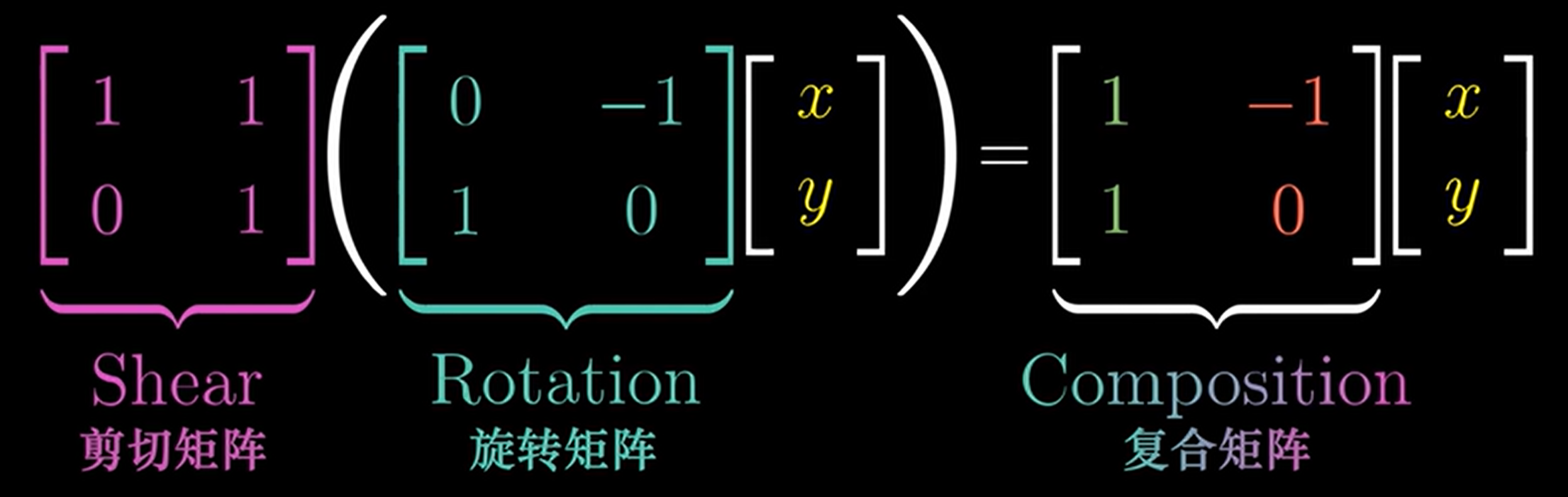
2. If the rank 1 matrix is not , you can consider calculating its square or cube;
Example: $\left(\begin{matrix}0&-1\\1&0\end{matrix}\right)^4=\left(\begin{matrix}1&0\\0&1\end{matrix}\right)$ Unit Formation <- After four operations, it becomes a unit Matrix;
3. If the matrix can be divided into a decomposition of the unit, then the matrix can be decomposed

4.3.1 Basic Operations of Matrices

Operation: Equal

$$A=(a_ij)_{m\times n}=B=(b_i)_{s\times k}\Leftrightarrow m=_S,n=k$$
and $a_{ij}=b_j(i=1,2,\cdots,m;j=1,2,\cdots,n)$, i.e., $A,B$ is a homomorphic matrix with equal elements.

Operations: Addition

When two matrices areisomorphic matrices, they can be added, that is:
$$C=A+B=\left(a_{ij}\right)_{m\times n}+\left(b_{ij}\right)_{m\times n}=\left(c_{ij}\right)_{m\times n}$$
$\text{ Among them, }c_{ij}=a_{ij}+b_{ij}(i=1,2,\cdots,m;j=1,2,\cdots,n),\text{ That is, the sum of the corresponding elements }$

Operations: Multiplication of numbers

Every element needs to be multiplied;
$$\begin{aligned}kA=Ak=&k\begin{bmatrix}a_{11}&a_{12}&\cdots&a_{1n}\\a_{21}&a_{22}&\cdots&a_{2n}\\\vdots&\vdots&&\vdots\\a_{m1}&a_{m2}&\cdots&a_{mn}\end{bmatrix}=\begin{bmatrix}ka_{11}&ka_{12}&\cdots&ka_{1n}\\ka_{21}&ka_{22}&\cdots&ka_{2n}\\\vdots&\vdots&&\vdots\\ka_{m1}&ka_{m2}&\cdots&ka_{mn}\end{bmatrix}\\&=\left(ka_{ij}\right)_{m\times n}\end{aligned}$$

Operations: Laws of operations - Multiplication/addition have commutative laws, associative laws, and distributive laws

$\text{ Commutative law }:\,A+B=B+A;$
$\text{ Associative law }:\,\left(A+B\right)+C=A+\left(B+C\right);$
$\text{ Distribution law }:\,k\left(A+B\right)=kA+kB,\left(k+l\right)A=kA+lA$
$\text{ The associative law of multiplication between numbers and matrices }:\,k\left(lA\right)=\left(kl\right)A=l\left(kA\right).$

Here, A，B，C is a homomorphic matrix, and k and l are arbitrary constants

4.3.2 Matrix Multiplication

#####Theorem: Matrixmultiplication

description: Multiplication of matrix Let $A$ be $m\times s$ matrix, $B$ be $s\times n$ matrix (the number of columns in matrix $A$ must equal the number of rows in matrix $B$), then $A$ and $B$ can be multiplied, and the product $AB$ is the $m\times n$ matrix, denoted as $C=AB=(c_ij)_{m\times n}$

The element $c_{ij}$ of the $i$-th row and column $j$ of > $C$ is the sum of the s elements in the $i$ row of $A$ and the $s$ pairwise elements in the $j$ column of $B$, that is:

$$c_{ij}=\sum_{k=1}^{s}a_{ik}b_{kj}=a_{i1}b_{1j}+a_{i2}b_{2j}+\cdots+a_{is}b_{sj}(i=1,2,\cdots,m;j=1,2,\cdots,n)$$

Explanation

Essence:
Multiplying two matrices actually manifests an operation:Each row of the left matrix multiplied by every column of the right matrix, andeach row multiplied by each column is the inner product of the vector(dot product operation)
The result of the inner product can reflect the magnitude of two vectors and the cosine of the angle between them;
Calculation:
Core:Decision row on the left, decision column on the right;
This is a multiplying type of multiplying multiple rows by columns, where each column in matrix A is multiplied by every row in B;
Since it is calculated by multiplying each column in A by every row in B, the number of columns in A must be equal to the number of rows in B;
That is: every element in the result of matrix multiplication is the result of the inner product;
$$\left(\alpha_{1}\alpha_{2}\right)^{T}\left(\alpha_{1}\alpha_{2}\right)=\left(\begin{matrix}\alpha_{1}^{T}\\\alpha_{2}^{T}\end{matrix}\right)\left(\alpha_{1}\alpha_{2}\right)=\left.\left(\begin{matrix}(\alpha_{1},\alpha_{1})&(\alpha_{1},\alpha_{2})\\(\alpha_{2},\alpha_{1})&(\alpha_{2},\alpha_{2})\end{matrix}\right.\right)$$
Example:
1. Many traveling and many rows: $\begin{pmatrix}a_{1}\\a_{2}\\a_{3}\end{pmatrix}(b_{1}b_{2}b_{3})=\begin{pmatrix}a_{1}b_{1}&a_{1}b_{2}&a_{1}b_{3}\\a_{2}b_{1}&a_{2}b_{2}&a_{2}b_{3}\\a_{3}b_{1}&a_{3}b_{2}&a_{3}b_{3}\end{pmatrix}$

Operations: The operational law of multiplication

Arithmetic Laws:
1. Associative law: to be satisfied
2. Distributive law: to satisfy or satisfy the situation
3. The associative law of multiplication and matrix product -> $(kA_{m\times s})B_{s\times n}=A_{m\times s}(kB_{s\times n})=k(A_{m\times s}B_{s\times n})$
Cannot be used:Does not satisfy the commutative law,Cancellation law cannot be used
1. Multiplication of matrices generally does not satisfy the commutative law, i.e., AB≠BA
For example: ABC and BAC are not necessarily equal;
2. There is $A\neq O, B\neq O, $ and $AB=O, $ therefore $AB=O\nRightarrow A=O$ or $B=O$
3. $AB=AC\Rightarrow A(B-C)=O,\text{ Even if there are such things at this moment, }A\neq O,\text{ Generally, you can't get it out of it }B=C$

Operations: Other rules of multiplication

（1）$\begin{aligned}&(A+B)^2=(A+B)(A+B)=A^2+AB+BA+B^2\neq A^2+2AB+B^2,\\&(A-B)^2=A^2-AB-BA+B^2\neq A^2-2AB+B^2,\end{aligned}$
（2）$\begin{aligned}&(A+B)(A-B)=A^{2}+BA-AB-B^{2}\neq A^{2}-B^{2},\\&(AB)^{m}=\overbrace{(AB)(AB)\cdots(AB)}^{m\uparrow}\neq A^{m}B^{m}.\end{aligned}$
(3) Important: A polynomial
$\text{ If }f\left(x\right)=a_{0}+a_{1}x+\cdotp\cdotp\cdotp+a_{m}x^{m},\text{ then }:\,f(A)=a_0E+a_1A+\cdots+a_mA^m$

4.3.3 Transpose Matrices

#####Definition: Transposethematrix

description: $\text{ General }m\times n\text{ Matrix }A=\left(a_{ij}\right)_{m\times n}\text{ The interchangeable row and column of }n\times m\text{ A matrix is called a matrix }A\text{ transpose matrix },\,\text{ Recorded as }A^T,\,\text{ That is }:\,$

$$A^{T}=\begin{bmatrix}a_{11}&a_{21}&\cdots&a_{m1}\\a_{12}&a_{22}&\cdots&a_{m2}\\\vdots&\vdots&&\vdots\\a_{1n}&a_{2n}&\cdots&a_{mn}\end{bmatrix}$$

Explanation

Write from line n to column n;
$A^{T}A$：
$$\left.A^{T}A=\left(\begin{matrix}a_{11}&a_{21}\\a_{12}&a_{22}\\a_{13}&a_{23}\end{matrix}\right.\right)_{3{2}}\left(\begin{matrix}a_{11}&a_{12}&a_{13}\\a_{22}&a_{12}&a_{23}\end{matrix}\right)_{{2}{3}}$$
Assume $\alpha_1=({a_{11},a_{21}})$, and other analogies, we get:
$$\left.\left(\begin{matrix}(\alpha_{1},\alpha_{1})&(\alpha_{1},\alpha_{2})&(\alpha_{1},\alpha_{3})\\(\alpha_{2},\alpha_{1})&(\alpha_{2},\alpha_{2})&(\alpha_{2},\alpha_{3})\\(\alpha_{3},\alpha_{1})&(\alpha_{3},\alpha_{2})&(\alpha_{3},\alpha_{3})\end{matrix}\right.\right)$$
This is a Gram matrix -> $A^{T}A$

Operations: The operational law of transpose matrices

$${(1)}\left(A^{\mathrm{T}}\right)^{\mathrm{T}}=A;\quad{(2)}\left(kA\right)^{\mathrm{T}}=kA^{\mathrm{T}};\quad{(3)}\left(A+B\right)^{\mathrm{T}}=A^{\mathrm{T}}+B^{\mathrm{T}};\quad{(4)}\left(AB\right)^{\mathrm{T}}=B^{\mathrm{T}}A^{\mathrm{T}}$$
Important: Principle of putting on and taking off
$(AB)^{\mathrm{T}}=B^{\mathrm{T}}A^{\mathrm{T}}$
Multiply from left to right, which equals writing from right to left: $\left(ABC\right)^{T}=C^{T}B^{T}A^{T}$

4.3.4 Determinant of a Phalanx

#####Definition: Determinantofaphalanx

description: $\text{ and should be employed }n\text{ The steps formed a square formation }A\text{ When calculating the determinant, denote as }|A|$;

1. $|kA|=k^{n}|A|\neq k|A|(n\geqslant2,k\neq0,1)$

2. $\text{ Generally, }\left|A+B\right|\neq\left|A\right|+\left|B\right|$

3. Note: $A\neq0\Rightarrow|A|\neq0$

4. $A\neq B\Rightarrow\left|A\right|\neq\left|B\right|$

5. $\left|A^{\mathrm{T}}\right|=\left|A\right|$

6. $\text{ Let }A,B\text{ This is a formation of the same rank, then }|AB|=|A||B|$

4.4 Several Important Matrices

4.4.1 Basic Matrix Form

Matrix One: Zero Matrix

Definition: A matrix where each element is zero, denoted as $O$

Matrix 2: Identity matrix

Definition:
A n-order square matrix where all main diagonal elements are 1 and all other elements are zero is called an n-order identity matrix, denoted as $E$ or $I$
Note: The way E is written
If it is $A_{32}$ and $B_{23}$
At this point: To calculate E-AB
Then $E$ should be written as $E_{3}$
At this point: To calculate E-BA
Then $E$ should be written as $E_{2}$

Matrix Three: scalar matrix

Definition:
The product of the number k and the identity matrix is called the scalar matrix
Formula:
$k\cdot E_{n}=\left.\left(\begin{matrix}k&\\&k&\\&&k\end{matrix}\right.\right)$
Features:
scalar matrices are commutative with any matrix multiplication: $k\cdot E\cdot A=A\cdot kE$

Matrix Four:(Key Point) Diagonal Matrix

Definition:
A matrix where all non-principal diagonal elements are zero is called a diagonal matrix;
That is: a matrix where all elements outside the main diagonal are 0
This is the simplified form of a matrix; a large number of matrices cannot be converted into this matrix;
Formula:
$A=\begin{pmatrix}\lambda_1&&&\\&\lambda_2&&\\&&\ddots&\\&&&\lambda_n\end{pmatrix}$

Matrix 5: Upper (lower) triangular matrix

Definition:
When $i>j$ or $i<j$ is, the matrix of $a_{ij}=0$ is called theupper triangular matrixorlower triangular matrix;

Matrix Six:(important) Symmetric matrices

Definition:
$$\text{ Conditions are met }A^\mathrm{T}=A\text{ The matrix }A\text{ This is called a symmetric matrix, }A^\mathrm{T}=A\Leftrightarrow a_{ij}=a_{ji}$$
Concept:
If a matrix is transposed and still itself after transposing, it is called a symmetric matrix;
Symmetry arrays have many inherent properties and are suitable for mathematical analysis;
Example:
$$\left(\begin{matrix}1&-2&1\\-2&0&3\\1&3&-1\end{matrix}\right)$$
Conclusion:
$\left(A^{T}A\right)^{T}=A^{T}\left(A^{T}\right)^{T}=A^{T}A$
Therefore: $A^{T}A$ must be a symmetric matrix. The form of a symmetric matrix can be used;

Matrix Seven: Antisymmetric matrix

Definition:
A matrix satisfying $A^T=-A$ $A$ called an antisymmetric matrix;
Formula:
$A^{\mathrm{T}}=-A\Leftrightarrow\begin{cases}a_{ij}=-a_{ji},i\neq j,\\a_{ii}=0.\end{cases}$
Concept:
The principal diagonal of the antisymmetric matrix must always be zero;
Example:
$\begin{pmatrix}0&-2&1\\2&0&3\\-1&-3&0\end{pmatrix}$

Matrix 8: Row matrix

A matrix with only one row of elements, also called a row vector;
In reality, it's a row with multiple columns;

Matrix Nine: Column matrix

A matrix with only one column of elements, also called a column vector;
In fact, it is one column with multiple rows;
Supplement:
Generally, write vectors, usually as column vectors;
You need to write the vector as a transpose to make the row vector work;
Supplements: $\alpha^T\alpha$ and $\alpha\alpha^T$
$\alpha^T\alpha$: Multiply 1n and n1 -> to get 1*1
$\alpha\alpha^T$: Multiply n1 and 1n -> to get n*n

Supplement: Rank 1 Phalanx

Example:
Given $\left(\begin{matrix}-1&-1&2\\2&2&-4\\1&1&-2\end{matrix}\right)$ to retrieve $\left(\begin{matrix}-1\\2\\1\end{matrix}\right)\left(1\quad 1\quad -2\right)$, its values must be proportional;
This type of matrix is called a rank 1 matrix;
In this matrix, the other two vectors can be represented by multiplying (1.1,-2) by 2 and -1 -> that is: its reference vector is one;
Therefore, it is a subspace within a three-dimensional vector;
Note:
A matrix of rank 1 does not necessarily mean a rank 1 matrix;
Nature:
For rank 1 matrix A, its $A^n=[tr(A)]^{n-1}$
For example: $A^3B=AAAB=[tr(A)]^2AB$

Additional Supplement: Matrix traces

Concept:
The sum of the principal diagonals of a matrix is called the trace of the matrix;
Symbol:
tr

4.4.2 Block Matrices

Concept: Segmentation of the matrix

Concept:
Using several vertical and horizontal lines to divide a matrix into several small pieces, each small piece called a subblock of the matrix;
Treat the subblock as an element of the original matrix to obtain the block matrix;
Block partitioning can reflect certain patterns within the matrix, allowing you to use these blocks to simplify calculations;
For example: $C=\left(\begin{matrix}A&O\\O&B\end{matrix}\right)$
Block by line according to A:
$$A=\begin{bmatrix}a_{11}&a_{12}&\cdots&a_{1n}\\\hline a_{21}&a_{22}&\cdots&a_{2n}\\\vdots&\vdots&&\vdots\\\hline a_{m1}&a_{m2}&\cdots&a_{mn}\end{bmatrix}=\begin{bmatrix}A_1\\A_2\\\vdots\\A_m\end{bmatrix}$$
Segment by column according to B:
$$B=\begin{bmatrix}b_{11}&b_{12}&\cdots&b_{1n}\\b_{21}&b_{22}&\cdots&b_{2n}\\\vdots&\vdots&&\vdots\\b_{m1}&b_{m2}&\cdots&b_{mn}\end{bmatrix}=\begin{bmatrix}B_1,B_2,\cdots,B_n\end{bmatrix}$$

Operations: Basic operations of block matrices (with 2*2 as an example)

Addition: $\text{ If the type is the same and the division method is consistent, then }\begin{bmatrix}A_1&A_2\\A_3&A_4\end{bmatrix}+\begin{bmatrix}B_1&B_2\\B_3&B_4\end{bmatrix}=\begin{bmatrix}A_1+B_1&A_2+B_2\\A_3+B_3&A_4+B_4\end{bmatrix}$
Note: The tangent of two matrices must be consistent, which equals the sum of each element;
Multiplication: $k\begin{bmatrix}A&B\\C&D\end{bmatrix}=\begin{bmatrix}kA&kB\\kC&kD\end{bmatrix}$
Multiplication: $\begin{bmatrix}A&B\\C&D\end{bmatrix}\begin{bmatrix}X&Y\\Z&W\end{bmatrix}=\begin{bmatrix}AX+BZ&AY+BW\\CX+DZ&CY+DW\end{bmatrix},\text{ It must be multiplier and can be added }$
Concept:
After chunking, treat it as an element, equivalent to multiplying two 2*2 matrices;
Note:
Because it is a matrix operation without commutative laws, the resulting result, such as $AX+BZ$, cannot change its order and cannot be written as $XA+BZ$
Note:
For multiplication operations, note that after multiplying blocks, the matrix on the left remains on the left, and the matrix on the right remains on the right;
If A and B are m, n-order square matrices respectively, then the power of the block diagonal matrix is:
Supplement:
$\begin{bmatrix}A&O\\O&B\end{bmatrix}^n=\begin{bmatrix}A^n&O\\O&B^n\end{bmatrix}$

4.5 Composite Transformations of Matrices

Example: Composite transformation of a matrix

Concept:
The matrix needs to be read from right to left because the function is written to the left of the variable: f(g(x))
Example: