Chapter 11: Multivariable Integral Calculus and Its Applications — Advanced Mathematics - Collection of Formulas
Chapter 11: Multivariable Integral Calculus and Its Applications from the formula collection, kept as a focused chapter for faster reading and image loading.
A binary function integrating along a two-dimensional curve segment;
Divide the curve into n small ends, multiply the curve's function value by the length of the small arc segment, sum each segment and take the limit. If this limit exists, then the line integral exists;
Theorem: Thefirsttypecalculatescurveintegrals: Direct method
Description: assume the parameter equation of L is $\begin{cases}x=\varphi(t),\\y=\psi(t),&\end{cases}(\alpha\leqslant t\leqslant\beta)$, then: $$\int_{L}f(x,y)\mathrm{d}s=\int_{\alpha}^{\beta}f(\varphi(t),\psi(t))\sqrt{\varphi'(t)^2+\psi'(t)^2}\mathrm{d}t$$
Explanation
Note:
ds is the arc derivative of the curve;
The upper and lower limits are arc lengths from small to large;
Theorem: Line integrals of the first kind in Cartesian coordinates
description: $\text{ If }C:y=y(x),\quad a\leq x\leq b$, then:
Divide the curve arbitrarily into n small ends, and multiply the projection of each directional small arc segment on the x-axis
Properties: Curves have direction; changing direction can alter symbols
$$\int_{L(AB)}Pdx+Qdy=-\int_{L(BA)}Pdx+Qdy$$
11.2.2 Calculation Methods
Method One: Direct Method
Theorem: Thesecondtypecalculatescurveintegrals
Description: If $L$ is parametrized by $\begin{cases}x=\varphi(t)\\y=\psi(t)\end{cases}$ and $t$ runs from $\alpha$ at the initial point $A$ to $\beta$ at the terminal point $B$, then $$\int_{L}P(x,y)\,dx+Q(x,y)\,dy = \int_{\alpha}^{\beta}[P(\varphi(t),\psi(t))\varphi^{\prime}(t)+Q(\varphi(t),\psi(t))\psi^{\prime}(t)]\,dt.$$
Explanation
Concept:
Write out the parameter equations, carry them in, and convert them into definite integral calculations;
Note:
The upper and lower limits are calculated from the starting point parameter -> the endpoint parameters, rather than by size;
Method 2: Green's Formula
On a double integral of a closed region D in a plane, can only the value difference on the boundary curve L be found without calculating the values of all points on the surface?
This function is achieved by Green's formula;
Definition: Singleconnectedarea
Description: A plane region $D$ is simply connected if every simple closed curve in $D$, together with its interior, lies entirely in $D$. Otherwise, the region is multiply connected.
Theorem: Greensformula
Description: Let the closed region $D$ be bounded by a piecewise smooth, positively oriented curve $L$. If $P(x,y)$ and $Q(x,y)$ have continuous first-order partial derivatives on $D$, then:
The range of Green's theorem used -> must be on a closed region: that is, the curve is closed;
The positive and negative directions are relative to the current area;
Where:
L is the positive boundary curve of region D;
Supplement: Closing an open path before applying Green's theorem
For an open path, add a convenient auxiliary segment to form a closed curve, apply Green's theorem, and then subtract the integral over the auxiliary segment.
(a) Change path: First, change to a simpler path (usually along the coordinate axis).
(b) Using a potential function: $\int_{(x_{1},y_{1})}^{(x_{2},y_{2})}P\mathrm{d}x+Q\mathrm{d}y=F(x_{2},y_{2})-F(x_{1},y_{1})$
Methods for finding the potential function: 1. Integrate one partial derivative and determine the remaining function; 2. Complete the total differential.
11.2.3 The Relationship Between Two Classes of Line Integrals
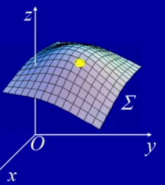
Example: Given that a curved surface component has a continuous surface density ρ(x, y, z), find its mass M;
Illustration
Multiply the density on each small area by its area, then sum them all to get the complete mass: $M=\lim_{\lambda\to0}\sum_{k=1}^n\rho(\xi_k,\eta_k,\zeta_k){\Delta S_k}$
Definition: Thefirstcategoryistheareaofcurves
description: $\text{ Let }\sum\text{ It is a smooth curved surface },f(x,y,z)\text{ It is defined as }\sum\text{ The first one }\text{ If }\Sigma\text{ Perform arbitrary segmentation and arbitrary local area point selection },$ can be obtained
Product sum limit: $\lim_{\lambda\to0}\sum_{k=1}^nf\left(\xi_k,\eta_k,\zeta_k\right)\Delta S_k$ exists in both cases, then this limit is called the function $f(x,y,z)$ the area component of the surface $\Sigma$ over the surface;
Written as: $$\iint_{\Sigma}f(x,y,z)dS=\lim_{\lambda\to0}\sum_{i=1}^{n}f(\xi_{i},\eta_{i},\zeta_{i})\Delta S_{i}$$
Explanation
Concept:
$ds$ Area equivalent to a small curved surface;
$f(x,y,z)$ Density equivalent to the surface of the surface;
$f(x,\gamma,z)\operatorname{d}S$ represents the mass of a small piece;
$\iint_{\Sigma}f(x,\gamma,z)\operatorname{d}S$ represents the sum limit for each small piece on the entire face;
$\Sigma$ Called the integration surface;
Explanation:
Multiply each function value by the area of its small surface element, sum, and take the limit. This first-kind surface integral is independent of orientation.
2. Existence of the surface part of the surface area: $\text{ If } f(x,y,z)\text{ On smooth curved surfaces }\sum\text{ Continuous on the upper stage }$, then the area component of the area of curvature exists;
3. Additivity to the integration domain: If $\sum$ is smooth in shards, then $\iint_{\Sigma}f(x,y,z)\operatorname{d}S=\iint_{\Sigma_{1}}f(x,y,z)\operatorname{d}S+\iint_{\Sigma_{2}}f(x,y,z)\operatorname{d}S$
4. Linear properties of integration: $$\begin{aligned}\iint_{\Sigma}[k_1f(x,y,z)\pm k_2g(x,y,z)]&\operatorname{d}S=k_1\iint_{\Sigma}f(x,y,z)\operatorname{d}S\pm k_2\iint_{\Sigma}g(x,y,z)\operatorname{d}S\end{aligned}$$
11.3.2 Calculation of Curvature Integrators of Area
Project the hard-to-find surface area onto a plane double integral on x and y to complete the calculation;
That is, project the surface $\sum$ onto $D_{xy}$ and convert it into a double integral on D;
${\text{ If a surface is defined by the equation }x}=x(y,z){\text{ or }\operatorname*{y}}=y(z,x)\text{ Given , it can similarly differentiate the area of a given area into corresponding parts }\text{ The double integral }$;
Conversion:
Substitute z with the expression about xy to get the double integral;
Note:
When a form like $x^2+y^2=1$ appears, where the central axis is the z axis, it cannot be done directly;
At this point, $y=y(x,z)$ -> $\iint_{\Sigma}f(x,y,{z}){\mathrm{d}S}=\iint_{D_{xy}}f(x,y=y(x,z),z)\sqrt{1+{z_x}^2(x,z)+{z_z}^2(x,z)}\mathrm{d}x\mathrm{d}z$ should be used
Similarly, for $x=x(y,z)$ form;
11.3.2.1 Parity and Symmetry
Theorem: Theparityofthefirsttypeofsurfacefraction
description: if the surface $\sum$ is symmetric about $xoy$, then:
Therefore, symmetry can be used to simplify the calculation: $\iint_{\Sigma}(x^2+y^2)ds=(\frac{2}{3})\iint (x^2+y^2+z^2)ds=(\frac{2}{3})\iint 1ds=\frac{2}{3}4\pi$
11.4 Surface Integrals of the Second Kind
11.4.1 Projection toward surfaces and surface elements
The surface specified on the side is called a directed surface, whose direction is represented by the direction of the normal vector
Let $\Sigma$ be the directed surface $, $ and the projection of its surface element $\Delta S$ on the $xOy$ surface is denoted as $\left(\Delta S\right)_{xy}$
11.4.2 Surface Integrals with Respect to Coordinates
Note: The second type of curved area has direction
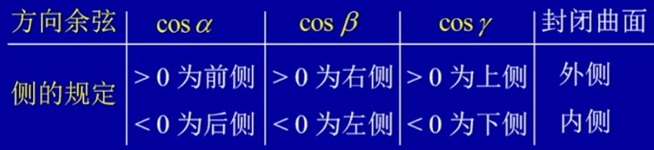
Concept: What is the orientation of a surface?
The direction of a surface is the lateral direction of the surface: if the normal direction is up, then the side faces up; if the normal direction is downward, then the side faces down;
Explanation:
The function value of a point $R(\xi_i,\eta_i,\zeta_i)$ multiplied by its projection on xy: $(\Delta S_i)_{xy}$
If it is $dxdy$ -> projection on xy;
If it is $dzdx$ -> projection on xz;
Properties: Related to the direction of the integrating surface
Change the direction of the surface, with opposite values;
Establish the relationship between the quadrilateral area of a closed surface and the threefold integral of the spatial body on the region enclosed by the surface;
In fact, it is a conclusion completely similar to Green's formula in the integral of curves;
Green's theorem establishes the relationship between the line integral of a closed curve in a plane and the double integral on the region enclosed by the closed curve;
Supplement: Use the Gaussian formula to cover the surface
When the surface is not closed, add a face using the Gaussian formula;
Then, the result calculated using Gauss's formula - is added to the added part;
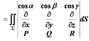
11.4.4 The Relationship Between Two Types of Curvature Divisions
Concept: The relationship between two types of curved area fractions