Chapter 6: Differential Equations

6.1 First-Order Differential Equations

Question Type 1: Separable variables

Format:
$$y^{\prime}=f(x)g(y)$$
Method:
$\frac{dy}{dx}=f(x)g(y)$ can be separated as $\frac{dy}{g(y)}=f(x)\,dx$; this is a separable differential equation.
Solutions of separable variables: Two-sided integral $$\int\frac{dy}{g(y)}=\int f(x)dx$$

Problem Type 2: First-order homogeneous equations

Format:
$$\frac{dy}{dx}=\varphi(\frac{y}{x})$$
Method:
Step zero: Organize into homogeneous equations with only $\frac{dy}{dx}$ on the left, i.e., $\frac{dy}{dx}=\varphi(\frac{y}{x})$;
Step one: Write down the $u=\frac{y}{x}$
Step 2: Since $y=xu$, after taking the derivative of y, we get $\frac{dy}{dx}=u+x\frac{du}{dx}$, which is the expression for $y^{\prime}=\frac{dy}{dx}=u+x\frac{du}{dx}=u+xu^{\prime}$;
Step 3: Substitute into the original differential equation to obtain $u+x\frac{du}{dx}=\varphi(u)$, which is separable.
That is: turn it into a separable variable and solve;

Problem Type 3: First-order linear equations

Format:
$$y^{\prime}+P(x)y=Q(x)$$
Method:
Organize into standard form with general solution formulas
$$y=e^{-\int p(x)dx}\left[\int Q(x)e^{\int p(x)dx}dx+C\right]$$

6.2 Second-Order Differential Equations

Problem Type 4: Second-order constant coefficient homogeneous equation

Format:
$$y^{\prime\prime}+py^{\prime}+qy=0$$
Method:
Step 1: Write the characteristic equation
Step 2: Find the characteristic roots.
Step 3: Write the corresponding general solution.
For two distinct real roots:
General solution: $y=C_1e^{r_1x}+C_2e^{r_2x}$
For a repeated real root:
General solution: $y=e^{rx}(C_1+C_2x)$
For conjugate complex roots $r_{1,2}=\alpha\pm i\beta$:
General solution: $y=e^{\alpha x}(C_1\cos\beta x+C_2\sin\beta x)$

Problem Type 5: Second-order linear nonhomogeneous equations with constant coefficients

Format:
Equation: $$y^{\prime\prime}+py^{\prime}+qy=f(x)$$
Two non-homogeneous terms:
1. $$f(x)=e^{\lambda x}P_m(x)$$
2. $$f (x)=e^{\alpha x}\left\lfloor P_{l}^{(1)}(x)\cos\beta x+P_{n}^{(2)}(x)\sin\beta x\right\rfloor$$

Summary: Method

1. Split the forcing term into components when necessary and find a particular solution for each component.
2. Find the general solution of the associated homogeneous equation.
Step 1: Write the characteristic equation
Step 2: Find the characteristic roots.
Step 3: Write the corresponding general solution.
Note:
In homogeneous general solutions, $e$ is $e^{r x}$, not $e^{\lambda x}$
Here $r$ denotes a characteristic root; it is distinct from the parameter $\lambda$ in the forcing term.
For a single real root:
General solution: $y=C_1e^{r_1x}$
For two distinct real roots:
General solution: $y=C_1e^{r_1x}+C_2e^{r_2x}$
For a repeated real root:
General solution: $y=e^{rx}(C_1+C_2x)$
For conjugate complex roots $r_{1,2}=\alpha\pm i\beta$:
Here $\beta$ is the magnitude of the imaginary part of the roots.
General solution: $y=e^{\alpha x}(C_1\cos\beta x+C_2\sin\beta x)$
3. Choose a trial particular solution $y^{*}$:
For each component, use a trial form such as $y^{}=x^{k}Q_{m}(x)e^{\lambda x}$ or $y^{}=x^{k}e^{\alpha x}\bigl[R_{m}^{(1)}(x)\cos\beta x+R_{m}^{(2)}(x)\sin\beta x\bigr]$.
4. Determine each part of the trial particular solution:
$e^{\lambda x}$ or $e^{\alpha x}$
-> Directly taken from the original expression -> and also set the value of this $\lambda$ or $\alpha$;
$Q_m(x)$
Based on the $P(x)$ situation, analyze:
If $P(x)$ is in case 1: $P_{m}(x)$
Observe the $P_{m}(x)$ of the original form
If it is a constant term, set to $a$;
If it is a linear term, set to $ax+b$;
If it is quadratic, set to $ax^2+bx+c$;
If $P(x)$ is case two: $\bigl[R_{m}^{(1)}(x)\cos\beta x+R_{m}^{(2)}(x)\sin\beta x\bigr]$
If both cos and sin exist:
Take the highest term between $P_{l}^{(1)}(x)$ and $P_{n}^{(2)}(x)$ in the original expression;
The original formula is $f (x)=e^{\alpha x}\left\lfloor P_{l}^{(1)}(x)\cos\beta x+P_{n}^{(2)}(x)\sin\beta x\right\rfloor$
If it is a constant term, set to $A\sin x+B\cos x$;
If it is a linear term, set it to $(Ax+B)\sin x+(Cx+D)\cos x$ similar to this form;
If only one of the sine or cosine terms appears:
Use its polynomial degree as the maximum degree, but include both sine and cosine terms in the trial solution.
$x^{k}$
Determine the $k$ of $x^{k}$:
If it's case one:
The value of $k$ is the multiplicity of $\lambda$ as a root of the characteristic equation of the associated homogeneous equation.
Example: If the characteristic roots are $r_1=3$ and $r_2=1$, while $\lambda=2$, then $\lambda$ is not a characteristic root, so $k=0$.
If it's case two:
Set $k$ equal to the multiplicity of $\alpha+i\beta$ as a characteristic root.
$\alpha$ from $e^{\alpha x}$, $\beta$ from trigonometric functions in $P_{l}^{(1)}(x)\cos\beta x+P_{n}^{(2)}(x)\sin\beta x$;
If $\alpha+i\beta$ is not a characteristic root, $k=0$; if it is a simple root, $k=1$; if it is a double root, $k=2$.
Note:
If $r_{1,2}=\pm1$, then $1$ and $-1$ are two distinct simple roots; the $\pm$ notation does not indicate a repeated root.
5. Determine the coefficient and any constant
(1) Determine the coefficients in the trial particular solution.
After setting the components of $y^{}$ earlier, since there are still coefficients to be determined in $y^{}$, replace the original equation with the set function, compare the coefficients of the same power at both ends, and then obtain the result of $y^{*}$;
If the current equation is $y^{\prime\prime}+y=\sin x$, you need to substitute $y({})$ and $y^{\prime\prime}()$ into the original equation, then compare the coefficients of the power at both ends to obtain the results of each coefficient in $y^{*}$;
(2) Determine the arbitrary constants $C_1$ and $C_2$.
Use the two initial or boundary conditions supplied in the problem, for example $f(0)=0$ and $f^{\prime}(0)=1$.
Substitute them into the complete general solution $y=y_h+y_p$ and solve for the constants.
6. For differential equations of order 3 or above, combine them as follows
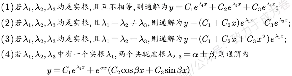
7. To obtain the solution satisfying specified initial or boundary conditions, substitute those conditions into the general solution and determine $C_1$ and $C_2$.
Supplement:
1. The difference of any two solutions of the same nonhomogeneous equation is a solution of the associated homogeneous equation.
2. Solutions to nonhomogeneous terms are superpositional;

Problem Type 6: $y^{\prime\prime}=f(x,y^{\prime})$ type descending equation

Format:
$$y^{\prime\prime}=f(x,y^{\prime})$$
Method:
Order: ${y^{\prime}=P,y^{\prime\prime}=\frac{dP}{dx}}$
Get: $\frac{dp}{dx}=f(x,p)$ First-order equations for p and x, then separate the variables;

Problem Type 7: $y"=f(y,y^{\prime})$ descending equation

Format:
$$y"=f(y,y^{\prime})$$
Method:
Set: $y^{\prime}=P$, $y^{\prime\prime}=\frac{dp}{dy}P$;
Become a first-order equation with only y and p and no x, then use the method of separating variables;