Lecture 38: Constant Coefficient Nonhomogeneous Linear Differential Equations

1.1 Nonhomogeneous Differential Equations

1.1.1 Basic Concepts

#####Definition: Constantcoefficientsfornonhomogeneouslineardifferentialequations

description:

1. Format: $$y^{\prime\prime}+py^{\prime}+qy=f(x)$$

2. Two non-homogeneous terms:

1. $$f(x)=e^{\lambda x}P_m(x)$$

2. $$f (x)=e^{\alpha x}\left\lfloor P_{l}^{(1)}(x)\cos\beta x+P_{n}^{(2)}(x)\sin\beta x\right\rfloor$$

Explanation

• Compared with the homogeneous constant-coefficient equation, the nonhomogeneous equation has an additional right-hand side:
• $y^{\prime\prime}+py^{\prime}+qy=f(x)$;
• The solution has two parts:
• general solution of the nonhomogeneous equation = general solution of the corresponding homogeneous equation + one particular solution;
• Common trial forms for a particular solution:
• Case 1: If $f(x)=e^{\lambda x}P_m(x)$, take
• $y^*=x^kQ_m(x)e^{\lambda x}$;
• Case 2: If $f(x)=e^{\alpha x}[P_l(x)\cos\beta x+Q_n(x)\sin\beta x]$, take
• $y^*=x^ke^{\alpha x}[R_m^{(1)}(x)\cos\beta x+R_m^{(2)}(x)\sin\beta x]$, where $m=\max\{l,n\}$;
• Case 3: If $f(x)$ is a sum of terms of these types, find a particular solution for each term and add them by superposition;

Summary of the Method

• 1. Split the right-hand side into components when necessary and choose a trial particular solution for each component;
• 2. Find the general solution of the corresponding homogeneous equation:
• Write the characteristic equation and find its roots;
• For one real root $r_1$: $y_h=C_1e^{r_1x}$;
• For distinct real roots $r_1,r_2$: $y_h=C_1e^{r_1x}+C_2e^{r_2x}$;
• For a repeated real root $r$: $y_h=e^{rx}(C_1+C_2x)$;
• For conjugate roots $r_{1,2}=\alpha\pm i\beta$: $y_h=e^{\alpha x}(C_1\cos\beta x+C_2\sin\beta x)$;
• 3. Choose the trial particular solution $y^*$:
• Use $y^=x^kQ_m(x)e^{\lambda x}$ or $y^=x^ke^{\alpha x}[R_m^{(1)}(x)\cos\beta x+R_m^{(2)}(x)\sin\beta x]$ as appropriate;
• 4. Determine each factor in the trial form:
• Copy $e^{\lambda x}$ or $e^{\alpha x}$ from the nonhomogeneous term;
• Give $Q_m(x)$ the same degree as $P_m(x)$: use $a$ for degree 0, $ax+b$ for degree 1, $ax^2+bx+c$ for degree 2, and so on;
• For trigonometric terms, include both sine and cosine with polynomial coefficients of degree $m=\max\{l,n\}$, even if only one appears on the right-hand side;
• Choose $k$ as the multiplicity of $\lambda$ (Case 1) or $\alpha+i\beta$ (Case 2) as a root of the characteristic equation. If it is not a root, $k=0$; for a simple root, $k=1$; for a double root, $k=2$;
• 5. Determine the coefficients and arbitrary constants:
• Substitute $y^$ and its derivatives into the original equation and compare coefficients to determine the unknown coefficients in $y^$;
• Add $y_h$ and $y^*$, then apply the initial or boundary conditions, such as $y(0)=0$ and $y^{\prime}(0)=1$, to determine $C_1,C_2$;
• 6. For equations of order 3 or higher, combine the homogeneous modes as shown below:
• 
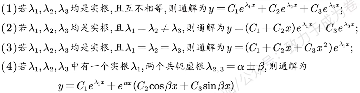
• 7. The resulting solution satisfying the given initial or boundary conditions is obtained after all arbitrary constants are determined;
• Supplement:
• The difference between any two particular solutions of the same nonhomogeneous equation is a solution of the corresponding homogeneous equation;
• Particular solutions obey superposition with respect to sums on the right-hand side;

1.1.2 Method Summary

Problem-Solving Steps

• Step 1: Form the characteristic equation and obtain (1) the homogeneous general solution;
• Step 2: Choose the correct trial particular solution $y^*$ from the type of the nonhomogeneous term;
• Step 3: Substitute the trial solution into the original equation;
• Step 4: Solve for (2) one particular solution of the nonhomogeneous equation;
• Step 5: Form (3) the nonhomogeneous general solution:
• nonhomogeneous general solution = homogeneous general solution + one particular solution.